Lecture notes: “Algebra and Polyhedral Geometry”
May 30, 2014 Anders Nedergaard Jensen Preface
This course is inspired by the book “Gr¨obner bases and convex polytopes” by Bernd Sturmfels [13]. Motivated by algorithmic problems for multivariate poly- nomial rings and polynomial equations we study Gr¨obner bases and their term orderings. Buchberger’s algorithm, convexity and Newton polytopes play im- portant roles. The theory is applied to toric ideals and integer programming.
Unexpectedly the combinatorial space of regular triangulations of a vector con- figuration naturally appears in this algebraic setting. The class will end with a brief introduction totropical geometry where all the theory is combined.
While Sturmfels’ book can be difficult to read for a beginner, the course notes “Computational Algebra and Combinatorics of Toric Ideals“ by Diane Maclagan and Rekha Thomas [11] are more accessible. Those notes are recom- mended when the lecture notes for our class are too brief.
We begin with an introduction to Gr¨obner bases since not everybody took an introductory algebra class based on Lauritzen’s book [10].
These notes, which will keep growing through the semester, can be found at
http://home.imf.au.dk/jensen/teaching/2014AlgebraAndPolyhedralGeometry/notes.pdf
while a version from the same class in 2012 can be found here
http://home.imf.au.dk/jensen/teaching/2012AlgebraAndPolyhedralGeometry/notes.pdf
The old version is complete, while the new version contains fewer mistakes.
Contents
1 Gr¨obner bases 4
1.1 The polynomial ring . . . 4
1.2 Monomial ideals and Dickson’s Lemma . . . 5
1.3 Term orderings . . . 7
1.4 Initial terms and initial forms . . . 9
1.5 The division algorithm . . . 9
1.6 Gr¨obner bases . . . 12
1.7 Buchberger’s Algorithm . . . 15
1.8 Elimination . . . 17
2 Lattices, convexity and Robbiano’s Theorem 20 2.1 Lattices . . . 20
2.2 Convexity . . . 23
2.3 Robbiano’s characterization of term orders . . . 24
3 Polyhedral geometry 27 3.1 Polyhedra . . . 27
3.2 Cone duality . . . 30
3.3 Dimension and faces . . . 32
3.4 Polyhedral complexes and fans . . . 35
4 The Gr¨obner fan of an ideal 40 4.1 Finiteness . . . 42
4.2 EveryC≺(I) is of the form Cv(I) . . . 42
4.3 Definition of the Gr¨obner fan . . . 44
4.4 Equivalence classes are relatively open cones . . . 45
4.5 The relative interior of a cone is an equivalence class . . . 48
4.6 The intersection of two Gr¨obner cones is a face of both . . . 49
5 Homogeneous ideals 51 5.1 Semigroups and monoids . . . 51
5.2 The semigroup ring . . . 51
5.3 Gradings and homogeneity . . . 52
5.4 Hilbert functions . . . 55
5.5 Homogeneity implies completeness . . . 56
5.6 Homogenisation . . . 57
5.7 Links in Gr¨obner fans . . . 59
5.8 “Very homogeneous” ideals . . . 61
5.9 The Gr¨obner walk . . . 63
6 Toric ideals 67 6.1 Saturation . . . 67
6.2 Lattice ideals . . . 69
6.3 Toric ideals . . . 71
6.4 Fibers and integer programming . . . 73
7 Regular triangulations and secondary fans 78
7.1 Simplicial complexes and Stanley-Reisner ideals . . . 78
7.2 Radical ideals . . . 79
7.3 Regular triangulations of vector configurations . . . 79
7.4 Sturmfels’ Theorem . . . 82
8 A brief introduction to tropical geometry 86 8.1 Tropical hypersurfaces . . . 86
8.2 Enumerative geometry . . . 87
8.3 Tropical varieties . . . 87
A Exercises 89 A.1 First sheet . . . 89
A.2 Second sheet . . . 90
A.3 Third sheet . . . 91
B Suggested projects 92 C Notation and conventions 94 D Software introductions 95 D.1 Singular . . . 95
D.2 Polymake . . . 96
D.3 Gfan . . . 97
E Exam topics 98
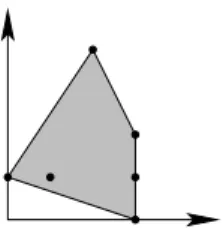
Figure 1: The Newton polytope of the polynomial in Example 1.1.3.
1 Gr¨ obner bases
In this section we define Gr¨obner bases and start discussing their relation to convex geometry. On our way we will have to define term orders, initial terms and the division algorithm.
1.1 The polynomial ring
We let k be a field and n ∈ N := {0,1,2, . . .} and consider the ring S :=
k[x1, . . . , xn] of polynomials in the variablesx1, . . . , xnwith coefficients ink. In examples we will often use letters as variable names, and for example consider the ringQ[x, y, z].
Definition 1.1.1 A vector u ∈ Nn defines the monomial xu := xu11· · ·xunn. The vectoru is called anexponent vector. By a term we mean a polynomial in k[x1, . . . , xn] of the formcxu with c∈k\ {0}.
If we require the exponent vectors to be distinct then a polynomial can be written uniquely as a sum of terms.
Definition 1.1.2 Thesupport supp(f) of a polynomialf ∈k[x1, . . . , xn] is the set of exponent vectors inf (in its unique representation). TheNewton polytope NP(f) is the convex hull of supp(f) in Rn.
For the precise definition of convex hull see Definition 2.2.2.
Example 1.1.3 The polynomial f = (x3+y+xy)−(1 +x3+x2) =y+xy− 1−x2∈Q[x, y] has supp(f) ={(0,1),(1,1),(0,0),(2,0)}. Its Newton polytope is shown in Figure 1.
Definition 1.1.4 For polynomials f, g ∈ k[x1, . . . , xn] we say that f divides g and write f|g if there exists h ∈ k[x1, . . . , xn] such that f h = g. We let g/f:=h.
We will be interested in ideals in the polynomial ringS (nonempty subsets of S which are closed under (1) addition (f, g ∈ I ⇒ f +g ∈ I), and (2) multiplication by elements inS (f ∈I∧g∈S ⇒ f g∈I)). Considering these sets as equations, they define subsets ofkn calledvarieties:
Definition 1.1.5 Let I ⊆k[x1, . . . , xn] be an ideal. Thevariety V(I) defined byI is
V(I) :={a∈kn:∀f ∈I :f(a) = 0}.
One way to get an ideal is to take a finite set of polynomialsf1, . . . , fm and look at the set they generate: hf1, . . . , fmi := {P
igifi : gi ∈ S}. This is an ideal. Even if we allow a possible infinite generating set of polynomials F ⊆ k[x1, . . . , xn] the set they generatehFi={Pm
i=0gifi :m∈N∧gi∈S∧fi ∈F} is an ideal. Hilbert’s basis theorem, which will follow from Proposition 1.6.7, says that a finite set of generators suffices:
Theorem 1.1.6 (Hilbert’s Basis Theorem) Let k be a field, n∈ N and I an ideal ink[x1, . . . , xn]. Then there exists a finite setf1, . . . , fm of polynomials such thatI =hf1, . . . , fmi.
Lemma 1.1.7 Let R be a commutative ring, and F ⊆R a generating set for an idealI :=hFi. IfI has a finite generating set G, then there is a finite subset F′ ⊆F such that I :=hF′i.
Proof. Each element inGcan be written as Pm
i=1gifi for somem∈N,gi ∈R, and fi ∈ F. We now take F′ to be the finite set of all fi appearing when expressing all elements ofGin this way. Then I =hGi ⊆ hF′i ⊆ hFi=I. 2
Recall that thequotient ringk[x1, . . . , xn]/I consists of elements of the form [f] :=f+I ={f+h:h∈I}wheref ∈k[x1, . . . , xn]. The element [f] is called acoset and together the cosets form a ring with operations [f] + [g] := [f +g]
and [f][g] := [f g]. Furthermore, [f] = [g] if and only if f−g∈I. We are interested in computational tools for the following problems:
• Finding all points in the varietyV(I).
• Doing computations in the quotient ring k[x1, . . . , xn]/I – In particular testing ideal membership: Givenf ∈S and generators for an idealI ⊆S, decide iff ∈I.
Gr¨obner bases will help us solve these problems. Furthermore, the existence of Gr¨obner bases will prove Hilbert’s basis theorem.
1.2 Monomial ideals and Dickson’s Lemma
In this subsection we consider the special case of monomial ideals.
Definition 1.2.1 An ideal I ⊆k[x1, . . . , xn] is called a monomial ideal if it is generated by (possibly infinitely many) monomials.
We observe that a polynomial belongs to a monomial ideal if and only if each of its terms does. Furthermore, a monomial ideal is determined by the set of monomials it contains (because these generate the ideal). This makes it possible to draw monomial ideals by drawing the exponents vectors of their generators inRn.
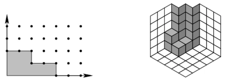
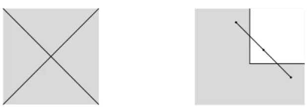
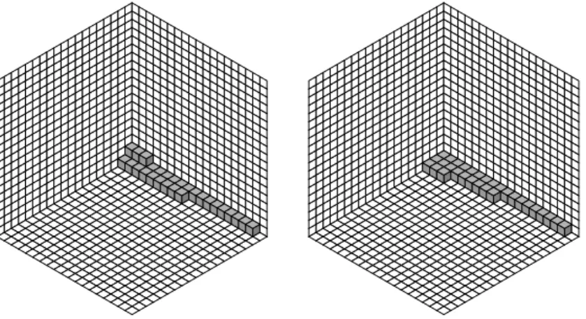
Figure 2: Staircase diagrams of the ideals in Example 1.2.2.
Observe that xv|xu if and only if∀i:vi ≤ui. Furthermore if M is a set a monomials thenxu ∈ hMi ⇔ ∃xv∈M :xv|xu. See Exercise 10, Sheet 1.
Example 1.2.2 Staircase diagrams of the monomial idealsI :=hx4, x2y, y2i ⊆ k[x, y] and J := hx2, y3, y2z2, xyzi ⊆ k[x, y, z] are shown in Figure 1.2. The second picture is drawn without perspective, and can therefore be interpreted in two ways. Most likely your mind will see the grey cubes with coordinates being vectors not among the exponent vectors of monomials inJ.
A generating setF ⊆k[x1, . . . , xn] for an ideal is calledminimal if for every f ∈F :hFi 6=hF\ {f}i.
Lemma 1.2.3 Every monomial ideal I ⊆k[x1, . . . , xn] has a unique minimal monomial generating set.
Proof. Consider the setF :={xu ∈I :∀xv ∈I\ {xu}:xv 6 |xu}. We first prove thatF generatesI by showing that every monomialxw ∈I is divisible by some element ofF. Ifxw∈F then indeed xw ∈F dividesxw. Ifxw6∈F then there existsxw′ ∈I\ {xw}such thatxw′|xw. Ifxw′ ∈F then we are done. Ifxw′ 6∈F then there exists xw′′ ∈ I \ {xw′} such that xw′′|xw′|xw. If xw′′ ∈ F then we are done. We continue in this way, but the process must eventually stop since the integer entries of the exponent vectors become smaller and smaller. Hence there existsxu ∈F such that xu|xw.
We now argue thatF is contained in any monomial generating set forI. But this is indeed the case because no other generator can divide these elements.
This shows thatF is minimal and unique. 2
We prove Hilbert’s basis theorem in the monomial case:
Lemma 1.2.4 (Dickson’s Lemma) Every monomial ideal I ⊆k[x1, . . . , xn] has a finite monomial generating set.
Proof. Induction. For n = 0 the ideal is either {0} or k. In the first case the empty set∅ is a finite generating set. In the second case {1} is.
For n > 0 we let π : Nn → Nn−1 denote the projection which forgets the last coordinate. Define E := π({v ∈ Nn : xv ∈ I}). By the induction hypothesis J :=hxu :u ∈Ei ⊆ k[x1, . . . , xn−1] has a finite generating set and
by Lemma 1.1.7 there exists a finite subset F ⊆E such thatJ =hxu :u∈Fi. Each u ∈ F has some lift v ∈ Nn such that π(v) = u and xv ∈ I with vn
minimal. We let Gdenote the set of these lifts. We now take m= maxv∈Gvn. Ifxw ∈I with wn> mthen the there is some u∈F such thatxu|xπ(w). Since wn > m the lift v of u satisfies xv|xw. Now for j = 0, . . . , m we consider the idealJj := hxu :u ∈Nn−1 and xuxjn ∈Ii ⊆ k[x1, . . . , xn−1]. Geometrically Jj
is a slice of (the complement of) the staircase diagram ofI whereun=j. By induction eachJj has a finite monomial generating set Gj. The set {xv :v ∈ G} ∪Sm
j=0{xuxjn:xu∈Gj} is a finite generating set ofI. 2
Corollary 1.2.5 LetM1⊆M2 ⊆M3 ⊆ · · · be monomial ideals ink[x1, . . . , xn].
For somej∈Nwe must have Mj =Mj+1 =Mj+2=· · ·. Proof. We consider the idealM :=S
iMigenerated by all monomials in allMi. By Lemma 1.2.4 it has a finite generating setF. For each fi ∈ F there exists a ji ∈ N such that fi ∈ Mji. For j := maxi(ji) we have F ⊆ Mj, implying M ⊆Mj. SinceMi ⊆M for all iwe have M =Mj =Mj+1 =· · ·. 2
A ring for which the above corollary holds for inclusions of any idealsI1⊆I2⊆
· · · (not necessarily monomial ideals) is called aNoetherian ring. We will prove later thatk[x1, . . . , xn] is Noetherian.
1.3 Term orderings
Recall that atotal ordering≤on a setXis a relation satisfying for alla, b, c∈X:
Antisymmetry: a≤b∧b≤aimpliesa=b.
Transitivity: a≤b∧b≤c implies a≤c.
Totality: a≤b∨b≤a.
Just like [11] and [13] we will be sloppy and sometimes forget the horisontal bar when writing ≤. For example when we say “Let ≺be a total order(ing)”
we really mean that should be the total ordering, and ≺is then defined by a≺b⇔ab∧a6=b.
Definition 1.3.1 Aterm ordering(or amonomial ordering)onk[x1, . . . , xn] is an total ordering on the monomials ink[x1, . . . , xn] such that:
• xaxb implies xaxc xbxc fora, b, c∈Nn.
• 1 =x0 xa for all a∈Nn.
Since term orders are orderings onmonomials, it would be more correct to call themmonomial orders and some people do that. However, as we shall see later, we most often use orderings to order the terms of a polynomial.
We give two examples of term orderings:
Example 1.3.2 We define thelexicographic term orderinglexonk[x1, . . . , xn] as follows. Fora, b∈Nnwe letxa≺lexxb ⇔a1< b1∨a1 =b1∧(a2 < b2∨a2= b2 ∧(. . .(an < bn). . .))). Or, more precisely, xa ≺lex xb ⇔ ∃j ≤ n : a1 = b1∧a2=b2∧ · · · ∧aj−1 =bj−1∧aj < bj.
Example 1.3.3 In Q[x, y, z] we have 1 ≺lex z ≺lex z2 ≺lex z9 ≺lex y ≺lex
yz2≺lexy5≺lexx2y2z≺lexx3.
Remark 1.3.4 For a, b ∈ Nn, xa lex xb if and only if a−b = 0 or the first non-zero entry ofa−b is negative.
Lemma 1.3.5 The lexicographic ordering ≺lex is a term ordering.
Proof. Antisymmetry: We havea, b∈Nnsuch thatxalex xbandxalexxb. Supposea6= b. Then Remark 1.3.4 says that the first non-zero entry of a−b is negative and the first non-zero entry ofb−ais negative. This is a contradiction. Hencexa=xb.
Transitivity: Suppose xa lex xb and xb lex xc. If a = b or b = c then we concludexalex xb. If botha6=bandb6=cthen by Remark 1.3.4 the first non-zero entry ofa−bis negative. So is the first non-zero entry ofb−c.
We conclude that the first non-zero entry of the sum (a−b)+(b−c) =a−c is negative, implyingxalexxc.
Totality: We havea, b∈Nn. Ifa=b thenxalexxb. Assumea6=bthen the first non-zero entry ofa−bis either positive or negative. In the last case xa lex xb. In the first the first case the first non-zero entry of b−a is negative, implyingxblexxa.
Multiplication respected: By Remark 1.3.4, xa lex xb is a condition on a−b. Furthermore,xa+clexxb+c is the same condition on (a+c)−(b+ c) =a−b.
1 is smallest: x0 lex xb since forb∈Nn, either 0−b= 0 or the first nonzero entry of 0−b is negative.
2
Example 1.3.6 We define the graded (or degree) reverse lexicographic term ordering ≺grlex on k[x1, . . . , xn] as follows. For a, b∈Nn we let xa≺grlexxb ⇔ P
iai <P
ibi∨P
iai =P
ibi∧ ∃j:aj > bj∧aj+1 =bj+1∧ · · · ∧an=bn. Lemma 1.3.7 Every term ordering ≺ onk[x1, . . . , xn] is a well ordering.
Proof. Let X be a set of monomials in k[x1, . . . , xn]. We must show that X contains a smallest element. By Lemma 1.2.4 and Lemma 1.1.7 the ideal hXi has a finite monomial generating setY ⊆X. Letxabe the smallest term in the finite setY. We claim that xa is a smallest element of X. Let xb be any term inX. Thenxb∈ hXi=hYi. Hence somexc ∈Y dividesxb. That is xb =xcxd for somed∈Nn. By Definition 1.3.1 we have 1xd, implyingxc xcxd=xb. We also havexaxc sincexc ∈Y. Hencexaxc xb as desired. 2
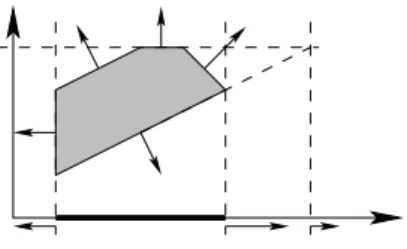
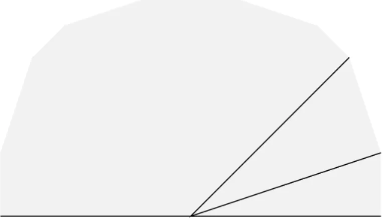
Figure 3: The Newton polytope off in Example 1.4.2.
1.4 Initial terms and initial forms
Definition 1.4.1 Let ≺ be a term ordering, ω ∈ Rn and f = P
u∈Ucuxu ∈ k[x1, . . . , xn] a polynomial with support U ⊆ Nn, cu 6= 0. If f 6= 0 we define theinitial term in≺(f) off to becuxu withxu being largest with respect to≺ among the monomials off. For anyf =P
u∈Ucuxu theinitial form inω(f) is the sum of allcuxu such thatω·u= maxv∈U(ω·v). We call maxv∈U(ω·v) the ω-degree of f.
When finding initial forms off it is advantageous to drawN P(f).
Example 1.4.2 Letf =x3−x3y+ 3x3y2+ 7x2y4−xy+y∈Q[x, y]. Then
• in≺lex(f) = 3x3y2,
• in(1,0)(f) =x3−x3y+ 3x3y2,
• in(100,1)(f) = 3x3y2,
• in≺grevlex(f) = 7x2y4, and
• in(1,1)(f) = 7x2y4. See Figure 3.
Lemma 1.4.3 Let ≺ be a term ordering, ω ∈ Rn and f, g ∈ k[x1, . . . , xn].
Then
• inω(f g) = inω(f)inω(g), and
• iff 6= 06=g then in≺(f g) = in≺(f)in≺(g).
Proof. Left to the reader. 2 1.5 The division algorithm
Ifn= 1 and we have only one generator for the idealI =hgi, then we can check if a given polynomial f is in I by running the well-known polynomial division algorithm onf, dividing by g. The remainder is 0 if and only if f ∈I.
In this section we generalize the division algorithm to more variables and more polynomials. Unfortunately, doing so, we loose the above important prop- erty. We can get a non-zero remainder even iff isI.
Algorithm 1.5.1 (Polynomial Division)
Input: A polynomial f ∈ k[x1, . . . , xn] and a list of polynomials {f1, . . . , fs} withfi ∈k[x1, . . . , xn]\ {0} and a term order ≺.
Output: A remainder r ∈ k[x1, . . . , xn] and a1, . . . , as ∈ k[x1, . . . , xn] such thatf =r+P
iaifi with no term of r divisible by any of in≺(f1), . . . ,in≺(fs).
Furthermore, iff 6= 0 then every termA of ai satisfies in≺(Afi)in≺(f).
• Fori= 1, . . . , s let ai := 0.
• Let r:= 0 and p:=f.
• While(p6= 0)
– Choose a term P from p. (For example P := in≺(p).) – If there existsi such thatin≺(fi)|P then
∗ ai:=ai+P/in≺(fi)
∗ p:=p−(P/in≺(fi))fi
– else
∗ r:=r+P
∗ p:=p−P
• Returnr, a1, . . . , as.
We notice that the division algorithm is non-deterministic since there may be more possible choices of P and i and the algorithm can choose as it likes.
In particular the output of the algorithm is not unique. Making the suggested choiceP := in≺(p) often makes the algorithm terminate sooner.
Proof. We prove correctness and termination. To prove that the algorithm is correct we must show that the output satisfies the specifications. We notice that the equation f = p+r+P
iaifi is satisfied at the beginning and after every iteration of the loop. At the endp= 0 and the equationf =r+P
iaifi follows. We also notice that only terms which are not divisible by any in≺(fi) are appended to r. Finally, notice that in≺(p) never gets ≺-larger during the algorithm: In the case where the condition of the if statement is true because in≺(P/in≺(fi)fi) = in≺(P/in≺(fi))in≺(fi) = (P/in≺(fi))in≺(fi) = in≺(P) in≺(p). In the second case because a term is removed from p. Consequently, any term P/in≺(fi) introduced to ai satisfies in≺((P/in≺(fi))fi) = in≺(P) in≺(p)in≺(f). Thus the output satisfies the specifications.
To prove that the algorithm terminates we observe that if we always make the choice P := in≺(p), then at each iteration the initial term in≺(p) keeps getting strictly smaller in the≺ordering: either because −in≺(P/in≺(fi)fi) =
−P cancels with P = in≺(p) or because P = in≺(p) is moved from p to r.
The set of in≺(p) appearing during a run of the algorithm must have a smallest element by Lemma 1.3.7. Hence the algorithm cannot continue forever.
If we do not consistently make the choice P := in≺(p) then the proof is trickier: We will first assume thatf is a single term. We letPidenote the value of P in the ith iteration, starting at i= 1,2, . . .. We now define a tree on the
set of is appearing, namely we connect i to j if Pj was introduced to p when processingPi. To be precise, we only connect itoj if the monomial of Pj was not present inp immediately before processingPi. This ensures thatj has just a single parent and that we therefore build a tree. We notice that Pj ≺ Pi if (i, j) is an edge. By Lemma 1.3.7 every path starting at the root must be finite.
By Lemma 1.5.2 below we get that the tree is finite. Hence the algorithm has to terminate. If f was not a single polynomial, then the argument still works by addingf as an artificial vertex 0 of the tree, and adding an edge from 0 to iifihas no parent. 2
Lemma 1.5.2 Let T be a tree with the property that any vertex v has only finitely many child vertices. Suppose that T does not contain an infinite path starting at the root. ThenT has only finitely many vertices.
Proof. Suppose thatT had an infinite number of vertices. We will construct an infinite path inT starting at the root v0. The root v0 has only finitely many children, so one of its children must have infinitely many vertices below it. Let’s call that childv1. We repeat the process withv1. Since there are infinitely many vertices below it, one of the childrenv2 has infinitely many vertices. The path v0, v1, v2, v2, . . . constructed in this way is infinite. This is a contradiction. 2 Example 1.5.3 Let≺=≺lex, f =x2y3−2y, f1=xy−y, f2 =x2y2−x−1, f3= x−2y+ 1. Here the initial terms have been underlined. We list some possible runs of the division algorithm. We keep track of the values p. A → means reducing by the subscript. A↓ means moving the subscript to the remainder.
• x2y3−2y→f1 xy3−2y→f1 y3−2y↓y3 −2y↓−2y 0 r=y3−2y
• x2y3−2y→f2 xy+y−2y=xy−y→f1 0 r= 0
• x2y3−2y ↓−2y x2y3 →f3 2xy4−xy3 →f1 2y4 −xy3 →f1 2y4 −y3 ↓−y3
2y4 ↓2y4 0 r = 2y4−y3−2y.
If we keep track of the coefficient polynomialsai in the second run, then we get the identityx2y3−2y =y(x2y2−x−1) + 1(xy−y) proving thatx2y2−2y∈ hxy−y, x2y2−x−1, x−2y+ 1i.
As the example shows, whether the remainder of the division is zero depends on the actual choices made in the algorithm. We would like to have a notion of
“reduces to zero” which is independent of the division algorithm:
Definition 1.5.4 Let f, f1, f2, . . . , fs ∈ k[x1, . . . , xn] be polynomials and ≺ a term ordering. We say that f reduces to zero modulo f1, . . . , fs if there exists a1, . . . , as such that f = P
iaifi and in≺(fi)in≺(ai) in≺(f) for all i with aifi 6= 0.
Lemma 1.5.5 If the remainder produced by some run of the division algorithm onf, f1, . . . , fs is 0 thenf reduces to zero modulo f1, . . . , fs.
Proof. Algorithm 1.5.1 produces the desired expression becausef = 0+P
iaifi. All we need to check is that forai 6= 0 we have in≺(fi)in≺(ai) in≺(f). But this also follows from the specifications of the algorithm. 2
1.6 Gr¨obner bases
Example 1.5.3 showed that the output of the division algorithm does not always have the desired properties. In this section we introduce the notion of Gr¨obner bases. We will see in Lemma 1.6.6 that Algorithm 1.5.1 is well-behaved if run with a Gr¨obner basis{f1, . . . , fs}.
Definition 1.6.1 Let I ⊆k[x1, . . . , xn] be an ideal. Let ≺be a term ordering andω ∈Rn. We define the initial ideals of I:
• in≺(I) :=hin≺(f) :f ∈I\ {0}iand
• inω(I) :=hinω(f) :f ∈Ii.
We observe that in≺(I) is always a monomial ideal, while inω(I) might not be:
Example 1.6.2 LetI :=hx2+y2+x2y, x2+xy+x2yi ⊆Q[x, y] andω= (1,1).
Then it is easy to see thatx2y is an initial form of an element of I and must be in inω(I). But actually x2y is not enough to generate inω(I). For example inω((x2 +y2+x2y)−(x2+xy+x2y)) = inω(y2−xy) =y2−xy. In fact we claim (without proof) that inω(I) =hy3, xy−y2, x3i. We also have in≺grlex(I) = hy3, xy, x3i.
As the example shows, it is not always easy to find the initial ideal. Later we will see how to do this for term orders (Algorithm 1.7.3) and vectors (Corol- lary 4.4.4).
Definition 1.6.3 Let I ⊆k[x1, . . . , xn] be an ideal and ≺be a term ordering.
A finite set{f1, . . . , fs} ⊆I is called aGr¨obner basis forI with respect to ≺if hin≺(f1), . . . ,in≺(fs)i= in≺(I).
Example 1.6.4 The set {x2+y2+x2y, x2+xy+x2y} is not a Gr¨obner basis for the ideal I in Example 1.6.2 with respect to ≺grlex since the initial forms of elements in the set are x2y = x2y. Which do not generate in≺grlex(I) = hy3, xy, x3i. The set{y3+y2+x2, xy−y2, x3+y2+x2} ⊆I is a Gr¨obner basis forI since its initial terms generate in≺grlex(I) =hy3, xy, x3i.
Lemma 1.6.5 If {f1, . . . , fs} is a Gr¨obner basis for an idealI ⊆k[x1, . . . , xn] with respect to a term order ≺thenI =hf1, . . . , fsi.
Proof. We need to show that I ⊆ hf1, . . . , fsi, so we pick f ∈ I. Let r be the remainder produced by a run of the division algorithm (Algorithm 1.5.1).
Notice that r ∈ I. Suppose that r 6= 0. Then the term in≺(r) ∈ in≺(I) = hin≺(f1), . . . ,in≺(fs)i. This means that some in≺(fi) divides in≺(r). This con- tradicts the properties of Algorithm 1.5.1. Hence r = 0, which implies that the polynomials produced in the algorithm satisfyf =r+P
iaifi =P
iaifi∈ hf1, . . . , fsi. 2
Lemma 1.6.6 Let{f1, . . . , fs}be a Gr¨obner basis for an idealI ⊆k[x1, . . . , xn] with respect to a term ordering ≺. The remainder produced by the division algorithm (Algorithm 1.5.1) when run on a polynomial f is independent of the choices performed in the run.
Proof. Suppose that one run gave r and another gave r′. Then r+P
iaifi = f =r′+P
ia′ifi imply r−r′ ∈I. Ifr6=r′ then there would be a leading term in≺(r −r′) ∈ in≺(I) which is not divisible by any in≺(fi). This contradicts hin≺(f1), . . . ,in≺(fs)i= in≺(I). 2
Gr¨obner bases have the properties we want. We first give a non-constructive proof of their existence. In the next section we present a concrete algorithm.
Proposition 1.6.7 Let I ⊆ k[x1, . . . , xn] be an ideal and ≺ a term ordering onk[x1, . . . , xn]. Then I has a Gr¨obner basis with respect to ≺.
Proof. The ideal in≺(I) is a monomial ideal. By Dickson’s Lemma 1.2.4 it has the formhxu1, . . . , xusi. By Exercise 10 of Sheet 1, for everyithere existsfi∈I such that in≺(fi) =xui. The set{f1, . . . , fs} ⊆I is a Gr¨obner basis ofI w.r.t.
≺because in≺(I) =hxu1, . . . , xusi=hin≺(f1), . . . ,in≺(fs)i. 2
In particular we have proved Hilbert’s Basis Theorem 1.1.6. Furthermore:
Corollary 1.6.8 For a field k the polynomial ringk[x1, . . . , xn]is Noetherian.
That is if I1 ⊆ I2 ⊆ I3. . . are ideals in k[x1, . . . , xn] then there exists j such thatIj =Ij+1=Ij+2 =· · ·.
Proof. We use the argument of the proof of Corollary 1.2.5. 2
Definition 1.6.9 Let I ⊆k[x1, . . . , xn] be an ideal and ≺a term ordering. A monomialxu6∈in≺(I) is called a standard monomial (w.r.t. I and ≺). We let std≺(I) denote the set of all standard monomials.
If we have a Gr¨obner basis for an ideal I one of the interpretations of the division algorithm is that it writes a polynomial f as a linear combination of standard monomials moduloI. The remainder is called the normal form of f. Lemma 1.6.10 The cosets of the standard monomialsstd≺(I)form ak-vector space basis {[xu] :xu ∈std≺(I)} of the quotient ring k[x1, . . . , xn]/I.
Proof. Let S = k[x1, . . . , xn]. To prove that the set spans S/I, take a vector [f]∈ S/I with f ∈ S. The Division Algorithm 1.5.1 gives an expression f = r+Ps
i=1aifi withr =P
xu∈std≺(I)cuxu and cu ∈k, implying f−Ps
i=1aifi= P
xu∈std≺(I)cuxu. Therefore [f] = [f −Ps
i=1aifi] = [P
xu∈std≺(I)cuxu] = P
xu∈std≺(I)cu[xu]. This proves that {[xu] :xu∈std≺(I)}spans S/I.
To prove independence of the set {[xu] : xu ∈ std≺(I)}, suppose that we had P
xu∈std≺(I)cu[xu] = [0] with cu ∈k. Then P
xu∈std≺(I)cuxu ∈I. If some cu was non-zero, then taking initial term we get a standard monomial in the initial ideal: in≺(P
xu∈std≺(I)cuxu) = cvxv ∈ in≺(I) for some v — a contra- diction. Thereforecu= 0 for all u and the vectors must be independent. 2
Corollary 1.6.11 Let{f1, . . . , fs}be a Gr¨obner basis for an idealI ⊆k[x1, . . . , xn] with respect to a term ordering ≺. A polynomial f belongs to I if and only if the remainder produced by the division algorithm is0.
Proof. If the remainder is 0, then we havef = 0 +P
iaifi ∈I. On the other hand, if f ∈ I then the remainder r produced by Algorithm 1.5.1 is a linear combination r = P
a∈std≺(I)caa with ca ∈ k and we have [0] = [f] = [r] = [P
a∈std≺(I)caa] = P
a∈std≺(I)ca[a] in k[x1, . . . , xn]/I. By Lemma 1.6.10 the standard monomials are independent, which shows ca = 0 for all a. Hence r= 0. 2
An ideal can have many Gr¨obner bases with respect to the same ordering as the following example shows.
Example 1.6.12 The idealI of Example 1.6.2 has
{y3+y2+x2,2xy−2y2, x3−x2y, x2y+x2+y2} ⊆I
as a Gr¨obner basis w.r.t. ≺grlex because the initial terms generate in≺grlex(I) = hx3, xy, y3i. Because in≺grlex(I) is generated by just the three monomialsx3, xy andy3, we can leave out x2y+x2+y2 and will still have a Gr¨obner basis:
{y3+y2+x2,2xy−2y2, x3−x2y} ⊆I.
This basis is called aminimalGr¨obner basis. We may also scale the polynomials to make the coefficients of the initial terms 1:
{y3+y2+x2, xy−y2, x3−x2y} ⊆I.
To get an even nicer Gr¨obner basis, we observe that thetail ofx3−x2y, being
−x2y, contains a monomial which is divisible by an initial term. We perform division of−x2ymodulo the polynomials and get the unique remainderx2+y2. We now substitute this tail, and get thereduced Gr¨obner basis
{y3+y2+x2, xy−y2, x3+x2+y2} ⊆I.
The precise definition of minimal and reduced follows below.
Definition 1.6.13 The Gr¨obner basis of Definition 1.6.3 is called minimal if if {in≺(f1), . . . ,in≺(fs)} is a minimal generating set for in≺(I). That is, no element can be left out. If furthermore, for every i no term of fi−in≺(fi) is divisible by any in≺(fj) and in≺(fi) has coefficient 1 then{f1, . . . , fs}is called areduced Gr¨obner basis.
Example 1.6.12 shows how to turn a Gr¨obner basis into a reduced one. We will later state these processes as Algorithms 1.7.8 and 1.7.9.
Proposition 1.6.14 Every ideal has at most one reduced Gr¨obner basis with respect to a given term order ≺.
Proof. By Lemma 1.2.3 the initial ideal in≺(I) has a unique minimal monomial generating set {xu1, . . . , xus}. Therefore every reduced Gr¨obner basis w.r.t. ≺ must consist of f1, . . . , fs where in≺(fi) = xui and all other monomials of fi
belong to std≺(I). Suppose there were two polynomials fi and fi′ in I with in≺(fi) = xui = in≺(fi′) and all other monomials in std≺(I). If fi −fi′ is non-zero, the monomial of in≺(f −f′) is in std≺(I) which is a contradiction.
Therefore there is only one possible choice offi. 2
The unique reduced Gr¨obner basis ofI with respect to≺is denoted G≺(I).
1.7 Buchberger’s Algorithm
Proposition 1.6.7 says that every ideal ideal I ⊆ k[x1, . . . , xn] has a Gr¨obner basis with respect to every term order. In this section we will show how to construct such a Gr¨obner basis given generators for I.
Definition 1.7.1 Let≺be a term order andf, g be two non-zero polynomials ink[x1, . . . , xn]. We define the S-polynomial of f and g:
S≺(f, g) = lcm(in≺(f),in≺(g))
in≺(f) f −lcm(in≺(f),in≺(g)) in≺(g) g where lcm(cxu, c′xv) :=xmax(u,v) (maximum is taken coordinate-wise).
We observe that the leading terms of the two parts of the S-polynomial cancel.
In particular, every term ofS≺(f, g) is≺-smaller than lcm(in≺(f),in≺(g)).
Theorem 1.7.2 Let G = {g1, . . . , gs} ⊆ k[x1, . . . , xn]\ {0} and ≺ be a term order. If for alli, j the polynomial S≺(gi, gj) reduces to zero modulo G, thenG is a Gr¨obner basis for I :=hGi.
Proof. Suppose G was not a Gr¨obner basis. Then there exists xu ∈ in≺(I)\ hin≺(g) : g ∈ Gi. By Exercise 10 of Sheet 1 there exists f ∈ hGi with xu = in≺(f). We may express f as a finite sum P
iaigi with ai being a term and the gi’s being (possibly repeated) elements of G. But let us not just pick an arbitrary such expression, but one where the largest in≺(aigi) appearing is smallest possible. This can be done since≺is a well-order (Lemma 1.3.7). Now consider a≺-largest termcxv = in≺(ajgj) appearing inP
iaigibefore summing up. This term must cancel since otherwise xu =xv ∈ hin≺(g) :g ∈Gi. Hence we find j′ with c′xv = in≺(aj′gj′). That the cancellation occurs implies that ajgj−cc′aj′gj′ is a multiple of S≺(gj, gj′) which reduces to zero, meaning that ajgj− cc′aj′gj′ = P
ldlfl for some fl ∈ G and dl with in≺(fldl) ≺ xv. In the sum P
iaigi we now replace ajgj by P
ldlfl and add cc′aj′ to the coefficient of gj′ (possibly making this summand disappear). This removes at least one appearance ofxv, and only introduces≺-smaller terms. We repeat this process until no more xv appear. We now have a contradiction since the expression P
iaigi forf has the largest terms≺-smallest, but we have an expression with smaller largest terms. Consequently,Gis a Gr¨obner basis with respect to≺. 2
Algorithm 1.7.3 (Buchberger’s Algorithm)
Input: A generating set F ={f1, . . . , ft} ⊆ k[x1, . . . , xn]\ {0} for an ideal I and a term order ≺.
Output: A Gr¨obner basis for I with respect to ≺.
• G:=F
• While ∃g, h∈G such thatS≺(g, h) does not reduce to zero moduloG.
– Letrbe a remainder produced by the division algorithm (Algorithm 1.5.1) run on S≺(g, h) and G
– Let G:=G∪ {r}.
Proof. To guarantee thatS≺(g, h) reduces to zero moduloGwe can use the Di- vision Algorithm 1.5.1 and Lemma 1.5.5. (A technical remark: If the remainder is non-zero then it is not clear thatS≺(g, h) does not reduce to zero modulo G.
However, it is clear thatGis not yet a Gr¨obner basis (Corollary 1.6.11) and it is safe to add the remainder toG, ensuring thatS≺(g, h) now reduces to zero.) If the algorithm terminates, then by Theorem 1.7.2 the set G is a Gr¨obner basis for hGi. Furthermore hGi=I since we only add elements of I to G. To show that the algorithm terminates we observe that in every step the monomial idealhin≺(g) : g ∈Gi keeps getting strictly larger because in≺(r) is produced from the division algorithm with the property that no in≺(g) divides it. By Corollary 1.2.5 this cannot go on forever. 2
Example 1.7.4 We continue Example 1.6.2, but starting with the generating set{g1, g2}={xy−y2, y3+x2+y2} forI and with≺being the degree reverse lexicographic ordering. To compute a Gr¨obner basis we first reduceS≺(g1, g2) =
−y4−x3−xy2 modulo{g1, g2}using the division algorithm and get remainder
−x3+y3 =: g3. Since the remainder is not zero, we add it to the generating set. We now check thatS≺(g1, g3) =−x2y2+y4 gives remainder zero modulo {g1, . . . , g3}. Finally we check that S≺(g2, g3) reduces to zero (possibly using Lemma 1.7.6 below). We conclude that {g1, . . . , g3} = {xy −y2, y3 +x2 + y2,−x3+y3} is a Gr¨obner basis. In particular in≺(I) =hxy, y3, x3i.
Remark 1.7.5 From the proof it follows that if we for some reason know that S≺(g, h) reduces to zero in the sense of Definition 1.5.4 then we can simply ignore that S-polynomial in the algorithm. The following lemma becomes useful.
Lemma 1.7.6 Let f, g∈k[x1, . . . , xn]\ {0} and ≺ a term ordering. If for all i:xi6 |in≺(f)∨xi6 |in≺(g) thenS≺(f, g) reduces to zero modulo f andg.
Proof. We observe thatS≺(sf, tg) =S≺(f, g) for s, t∈k\ {0}. Hence, we may assume that the coefficients of in≺(f) and in≺(g) are both 1. We then have
S≺(f, g) = lcm(in≺(f),in≺(g))
in≺(f) f −lcm(in≺(f),in≺(g)) in≺(g) g
= in≺(f)in≺(g)
in≺(f) f−in≺(f)in≺(g)
in≺(g) g= in≺(g)f−in≺(f)g
= (in≺(g)f−gf)−(in≺(f)g−gf) = (f−in≺(f))g−(g−in≺(g))f.
By to Definition 1.5.4 we are done if f or g is a single term. If not it suffices argue that in≺((f−in≺(f))g) and in≺((g−in≺(g))f) are smaller than or equal to in≺(S≺(f, g)) in the ≺ ordering. If the exponents of in≺((f −in≺(f))g) = in≺(f−in≺(f))in≺(g) and in≺((g−in≺(g))f) = in≺(g−in≺(g))in≺(f) are equal, then we conclude (using the assumption that in≺(f) and in≺(g) have no common monomial factor) that in≺(f)|in≺(f−in≺(f)). This contradicts the properties of ≺ being a term order. Hence in≺((f −in≺(f))g) and in≺((g −in≺(g))f) have different exponent vectors and the largest of these cannot cancel when subtracting. Therefore the largest term also appears inS≺(f, g). 2
Example 1.7.7 Using Lemma 1.7.6 it is easy to check that{x2+2xy+y3,3y2+ 3x+ 5} is a Gr¨obner basis with respect to≺(5,3)t.
It is common to extend Buchberger’s algorithm with the following two steps to compute the reduced Gr¨obner basisG≺(I), thereby making the output unique.
Algorithm 1.7.8 (Minimizing a Gr¨obner basis)
Input: A Gr¨obner basisG⊆k[x1, . . . , xn] w.r.t. some term order≺. Output: A minimal Gr¨obner basis G′ for hGi w.r.t. ≺.
• G′ :=G
• While it is possible to remove ag∈G′ fromG′, and still keep the equality hin≺(g) :g∈Gi=hin≺(g) :g∈G′i, do so.
Proof. The set remains a Gr¨obner basis for hGi since hin≺(g) : g ∈ G′i = in≺hGi. It is minimal since no further g can be deleted. 2
Algorithm 1.7.9 (Autoreducing a Gr¨obner basis)
Input: A minimal Gr¨obner basisG′ ⊆k[x1, . . . , xn]w.r.t. some term order≺. Output: The reduced Gr¨obner basis G≺(hG′i).
• Substitute each g ∈ G′ by in≺(g) +r, where r is the unique remainder produced by Algorithm 1.5.1 when run on the tailg−in≺(g) and G′. 1.8 Elimination
In Section 1.1 we stated three problems for polynomial rings which can be solved using Gr¨obner bases. We have already proved Hilbert’s Basis Theorem 1.1.6 and shown how Gr¨obner bases can be used to compute in the quotient ring k[x1, . . . , xn]/I (Corollary 1.6.11 and Exercise 5 on Sheet 2). We will now discuss how to solve polynomial equations. The technique presented works particularly well if the equations have only finitely many solutions over C.
Proposition 1.8.1 Let I ⊆k[x1, . . . , xn]be an ideal. LetGbe a Gr¨obner basis of I with respect to ≺lex. For l= 1, . . . , n we have G′ :=G∩k[xl, . . . , xn] is a Gr¨obner basis for the elimination ideal I∩k[xl, . . . , xn]⊆k[xl, . . . , xn].
Proof. Clearly, G′ ⊆ I ∩k[xl, . . . , xn] and hin≺lex(g) : g ∈ G′i ⊆ in≺lex(I ∩ k[xl, . . . , xn]). It remains to show that hin≺lex(g) : g ∈ G′i ⊇ in≺lex(I ∩ k[xl, . . . , xn]). Let xu be a monomial in in≺lex(I ∩k[xl, . . . , xn]). Then xu ∈ in≺lex(I). Since G is a Gr¨obner basis, there must exist g ∈ G such that in≺lex(g)|xu. Since xu contains no xj with j < l, this must also be the case for in≺lex(g). By the properties of the term order, no term from g can contain anxj withj < l. Henceg∈G′, provingxu ∈ hin≺lex(g) :g∈G′i. 2
We can use Gr¨obner bases for solving polynomial equations:
Example 1.8.2 We wish to compute the solutions to the system x2+y2 = 1 and x2+y2−x−y = 2. Let I =hx2+y2−1, x2+y2−x−y−2i ⊆ C[x, y].
We compute the lexicographic Gr¨obner basis {y2+y, x+ 1 +y}
(which is an equivalent system of equations) and conclude that I ∩C[y] = hy2+yi. From this we conclude thaty= 0 or y=−1. Substituting we get
V(I) ={(−1,0),(0,−1)}.
Why did every solution of the elimination ideal extend to a solution of the ideal?
We show two examples where this is not the case:
Example 1.8.3 The set{y2−y, xy−y, x2+ 1−2y}is a lexicographic Gr¨obner basis for an idealI ⊆R[x, y]. We solvey2−y= 0 and see thaty= 0 andy= 1 are solutions. The point (1,1) is in V(I) ⊆R2. However, there is no solution withy= 0 over the real numbers.
Example 1.8.4 LetI =hxy−1i ⊆C[x, y]. The generator is already a lexico- graphic Gr¨obner basis. We conclude that I∩C[y] =h∅i={0}. Any choice of y gives a solution to the elimination ideal. If we choose a value for y then the equationxy−1 = 0 tells us the value ofx. However, ify = 0 was chosen there is no solution forx.
The first example shows that the ideal must be algebraically closed for all solutions to extend, while the second shows that it is possible that not every point lifts in the case where we have more solutions than a finite set of points.
In the rest of this subsection we use the complex numbersC, but any alge- braically closed field will suffice. We will use the following classic result without proof:
Theorem 1.8.5 (Hilbert’s Nullstellensatz) Let I ⊆ C[x1, . . . , xn] be an ideal. If f ∈C[x1, . . . , xn]is zero on all points in V(I)then there exists N ∈N such thatfN ∈I.
Corollary 1.8.6 Let I ⊆ C[x1, . . . , xn] be an ideal and ≺ a term ordering.
Then V(I) ⊆ Cn is a finite set ⇔ dimC(C[x1, . . . , xn]/I) <∞ ⇔ |std≺(I)|<
∞.
Proof. The last two statements are equivalent because the standard monomials form a vector space basis of C[x1, . . . , xn]/I by Lemma 1.6.10. If V(I) ⊆ Cn is infinite and dimC(C[x1, . . . , xn]/I) =: d finite then we choose d+ 1 point in V(I) and for each point pi we construct a polynomial fi ∈ C[x1, . . . , xn] which take the value 1 atpi and zero on all other chosen points. These d+ 1 polynomials are linearly independent inC[x1, . . . , xn]/I since allf ∈I vanishes at the points. This contradicts the space having dimensiond.
On the other hand suppose V(I) ⊆ Cn is finite. For each coordinate di- rection xi we choose a polynomial fi ∈ C[xi] being zero on the projection of V(I) to that coordinate. We also have that fi is zero on V(I). By Hilbert’s Nullstellensatz there exists Ni ∈ N such that fiNi ∈ I. The term in≺(f) only involves the variable xi. Therefore, the ith exponent of standard monomial in std≺(I) is bounded. Since this holds on all coordinates xi, there can be only finitely many standard monomial. 2
Corollary 1.8.7 LetI ⊆C[x1, . . . , xn]be an ideal withdimC(C[x1, . . . , xn]/I)<
∞ and J = I∩C[xn]. If an ∈ V(J) ⊆ C1 then there exists a1, . . . , an−1 ∈ C such that(a1, . . . , an)∈V(I)⊆Cn.
Proof. The varietyV(I) is finite set of points, and so is the projection of these points onto the last coordinate. Letp1, . . . , pm be these projected points. The polynomial f =Qm
i=1(xn−pi) is zero on the projected points. If an does not lift, thenf is non-zero onan. The polynomial is zero on all points inV(I) and by Hilbert’s Nullstellensatz there exists N ∈ N such that fN ∈ I. It follows thatfN ∈J. ButfN(an)6= 0. This contradicts thatan∈V(J). 2
In general the elimination ideal defines the “Zariski closure” of the projection of V(I). Even with the limitations described above, lexicographic Gr¨obner bases are the first choice of tool for solving polynomial systems algebraically.
2 Lattices, convexity and Robbiano’s Theorem
We have seen in Exercise 7 of Sheet 1 that vectors can be used to construct termorders. In this section we will prove Theorem 2.3.5 which says that every termorder can be represented by a matrix.
2.1 Lattices
In this section we introduce lattices. They will be important later for toric ideals, lattice ideals, integer programming and Robbiano’s characterisation of term orders. Typically a lattice will sit inside someRn as a subgroup.
Definition 2.1.1 A group Lis called a lattice if it is isomorphic to the group Zm for some m ∈ N. The rank of the lattice is the number m. A set {b1, . . . , bm} ⊆L is called a(lattice) basis forL ifL={P
iaibi :ai ∈Z}. Given a subset B ⊆ Zn we let hBi denote the smallest subgroup of Zn containing B. We call B a generating set for hBi. We will prove that hBi is a lattice (Theorem 2.1.2) and see how to compute a lattice basis in case B is finite (Algorithm 2.1.6).
Theorem 2.1.2 Every subgroup G⊆Zn is a lattice of rank at most n.
Proof. Let for i= 1, . . . , m the function πi :Zn→ Z be the projection on the ith coordinate andSi :=πi(G∩({0}i−1×Zn−i+1)). Fori= 1, . . . , mifSi6={0} we construct abi as follows and collect these in a set B. The group Si ⊆Z is generated by one element a∈Z (as a ringZ is a principal ideal domain). We choosebi ∈G∩({0}i−1×Zn−i+1) such thatπi(bi) =a. In this way we construct at mostn vectorsbi. We claim that hBi=Gand the vectors are independent.
This would prove thatG is isomorphic toZm with m=|B| ≤n.
To show that B is independent, let P
j∈Jcjbj = 0 be a dependency with cj ∈ Z\ {0} and J 6= ∅ minimal. Let j′ be the smallest element of J. We have that the j′th coordinate of bj′ is non-zero by construction. But this is a contradiction, since all otherbj in the sum are zero on the j′th coordinate.
To show thatB generatesG, suppose not and letibe the largest index such thatG∩({0}i−1×Zn−i+1)\ hBi 6=∅, and pick an elementv in the difference.
Sinceiis largestvi 6= 0 and thereforeSi 6={0}meaning that we have introduced abi toB. We now subtractbi a suitable number of times fromv to get v′ with v′i= 0 and v′ ∈({0}i−1×Zn−i+1)\B contradicting the maximality ofi. 2 Remark 2.1.3 For the experts: Every submodule of a free module of rank n over a principal ideal domain is free with rank at most n. The proof is a straight forward generalization of the proof above. Important is that the ring is a principal ideal domain. In the following we will need that the ring is a Euclidean domain which is a slightly stronger condition.
In the rest of this section we explain the theorem by doing computations with lattices using the Gauss elimination algorithm over the integers.